SMIAR - Santa Margarita Infrasound Array

By Kris Walker, SIO/IGPP

Southern California is acoustically noisy. This noise comes from a variety of natural and human sources. We are interested in this noise, which in part comprises low-frequency sound waves called "infrasound" and gravity waves in the 0.001 - 10 Hz frequency band.

We have been interested in regional sources of infrasound in the Southern California region for a variety of reasons for many years. First, being physically close to these sources helps us learn more about the physics involved in how these sources generate infrasound. There are also many interesting hypotheses regarding the atmospheric influences on infrasound propagation that require testing by analyzing a large data set of observed infrasound signals from known source locations. We also need many infrasound signals from known source locations to test software that we are developing for analyzing infrasound and seismic signals that are buried in background noise and for modeling the propagation of infrasound signals. Finally, a nuclear monitoring infrasound array called "I57US" exists in Southern California (Figure 1). This array is part of the CTBTO International Monitoring System. Knowledge of regional sources of infrasound can help those who scan I57US data to distinguish between signals from regional sources and signals of interest that originate from other parts of the world.

We operate three infrasound arrays in Southern California (Figure 1). This document describes the Santa Margarita Infrasound Array (SMIAR), installed during the spring of 2010 and located about 5 miles to the southwest of Temecula, California.

Figure 1. Google Earth image of the Southern California Infrasound Network (SCIN). The green squares delineate the locations of contributing infrasound arrays. Each array contains six to nine low-frequency microphones called "microbarometers". These extremely sensitive "ears" listen for sounds in the 0.001 to 20 Hz range, which is well below the frequency threshold for human ears (18 Hz). This document describes the Santa Margarita Infrasound Array (SMIAR).

SMIAR comprises nine low-frequency microphones (called "MB2000 microbarometers") that measure changes in atmospheric pressure. The standard frequency range of these sensors is 0.01-27 Hz. However, they can also record large pressure signals down to 0.001 Hz, which makes them sensitive to other types of low-frequency phenomena like gravity waves and "solitons." The SMIAR microbarometers are laid out in a semi-irregular grid over a distance of roughly half a mile (775 m; Figure 2). One question you might have is "why do you need nine sensors?" We use nine sensors located in different places because that permits us to see how a signal moved across the array, which then permits us to determine the direction that the signal came from (pointing us toward the source). Infrasound travels at about 340 m/s (760 mph) at grazing angles to the Earth's surface. So a signal observed by one of these sensors will be delayed by one or two seconds before it is observed by the other sensors a few hundred meters away. This delay is easy to detect with modern technology and can even be observed visually as you will be see below.

Figure 2. Google Earth image of the SMIAR microbarometer locations. An MB2000 microbarometer is located at each black circle. Three MB2000's are connected to each Reftek 130 digitizer (red squares). Infrasound energy is converted to electrical energy by the microphone. The electrical energy travels up to 150 m over signal cable to the Reftek digitizer, where it is transformed to a digital format and sent over the Internet to our lab at UCSD in real time. The data are then scanned by a computer program to detect and characterize signals of interest.

Although MB2000 microbarometers are sensitive to ground motion, and earthquakes signals are routinely observed by these sensors, this does not generally affect their performance at this location. While it is true that several earthquake signals a month are registered here, we use standard computer programs to distinguish between these earthquake signals and real infrasound signals.

Construction (February - June 2010)

SMIAR planning began in early 2008. In the summer of 2009, we kindly received permission from SDSU to install the array.

Figure 3. View across the northern gorge looking south. Photo taken July 17, 2010.

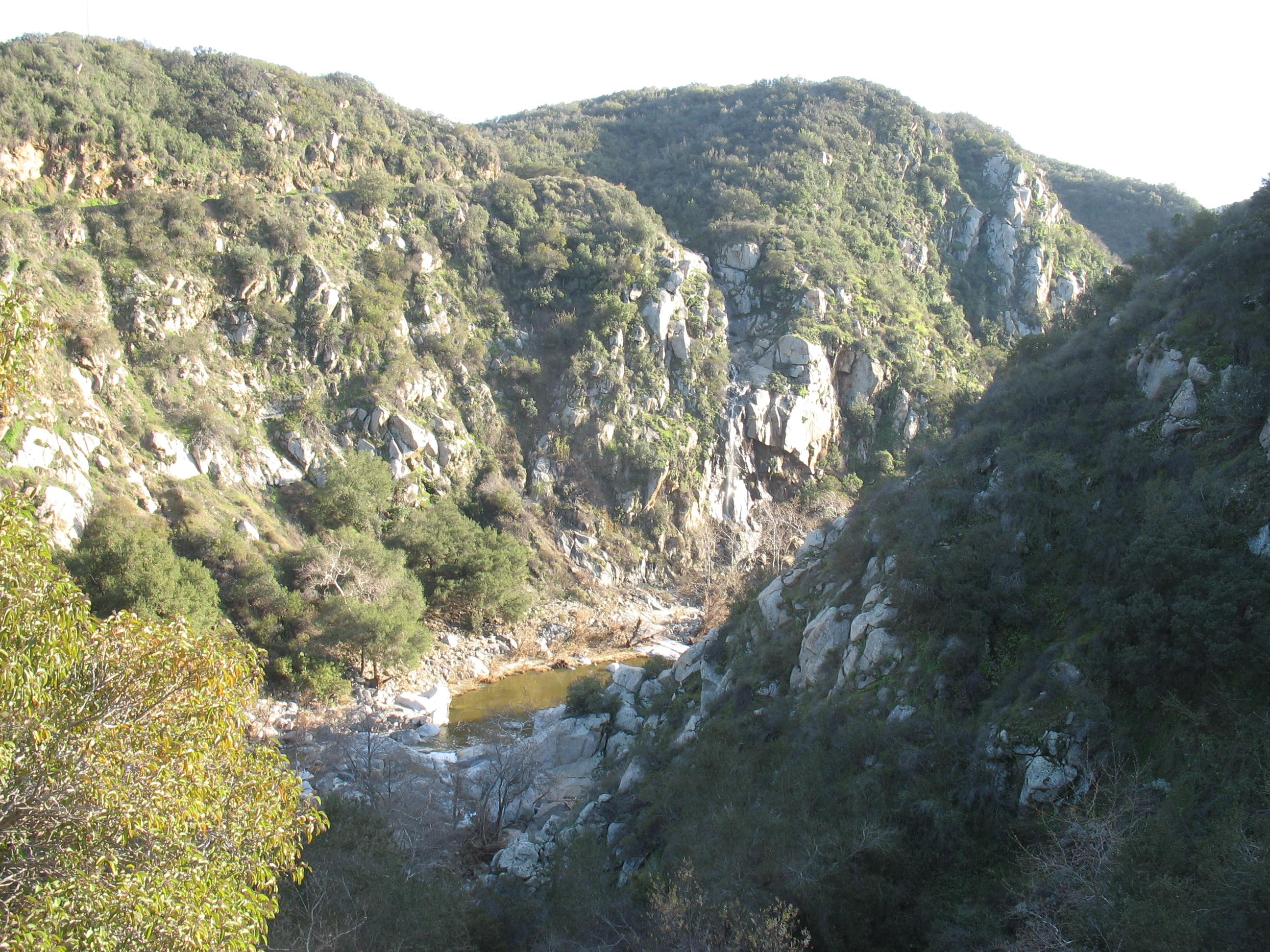
Santa Margarita Ecological Reserve is a beautiful jewel in Southern California (Figure 3). It seems that hundreds of different types of plants and animals call this place home. The landscape is covered by chaparral ranging in thickness and height up to 20 feet tall. This chaparral is good because it provides us with protection from the wind, which creates noise on our microbarometers. The chaparral is also home to many; we saw interesting birds, rodents, snakes, and plants. We also encountered countless, less interesting bees, flies, and biting bugs. The rocks in this area are part of the uplifted coastal range batholith, which seems to be wormy granitic gneiss.

Figure 4. Guided by Google Earth and a nine-sensor configuration plan, the first site survey to identify locations for digitizers. Photo taken July 17, 2009.

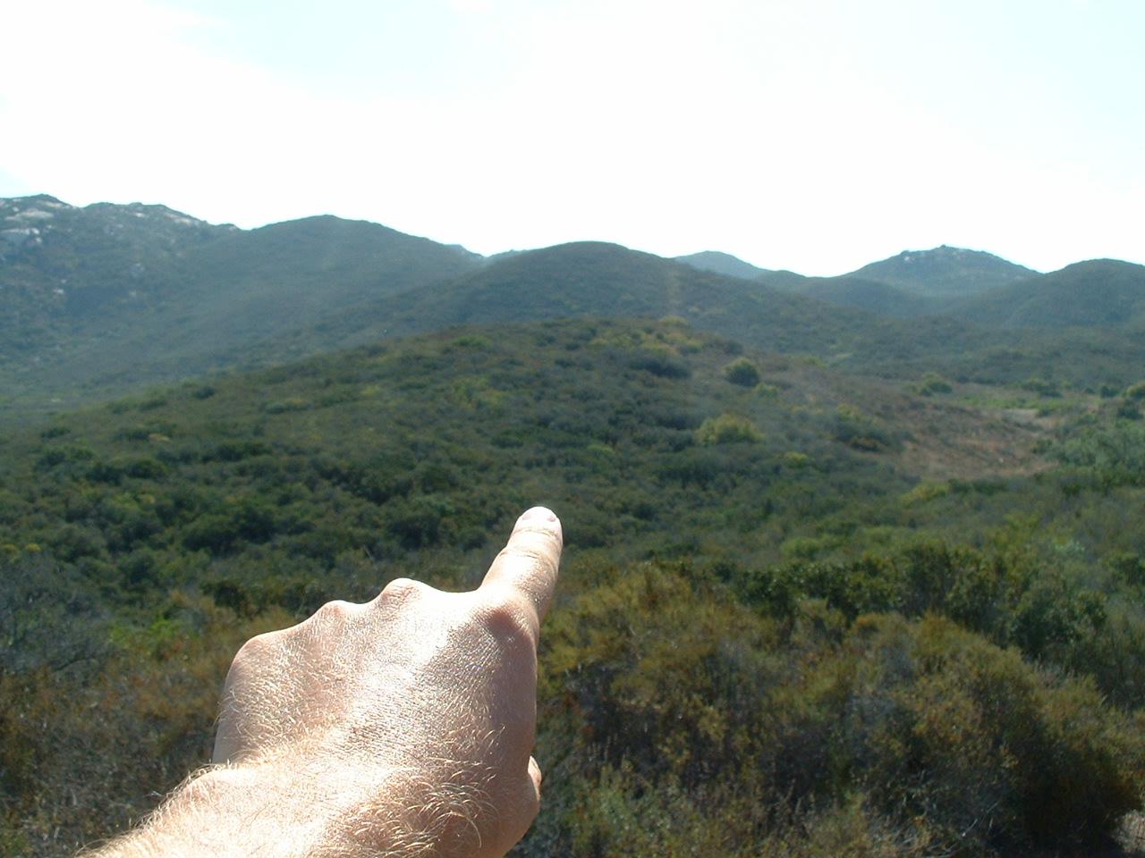
Sites were chosen for the three digitizers and nine sensors during the summer of 2009 (Figure 4). We received permission to install our array in January 2010. The maximum predicted trail length was 150 m. The first step was determining if onsite electromagnetic (EM) noise permitted such long signal cables between the digitizer and sensors. We did some onsite experiments (Figure 5) with two different cable types: Belden 8162 (expensive, twisted, multiple shielding) and Belden 8723 (less expensive with less shielding). We found that for 300 m cable lengths not in conduit, the 8162 cable is much quieter (picked up less EM noise). For 120 m cable inside steel-reinforced liquid tight (LT) conduit, there was no difference in EM noise between the two cable types. So we chose the 8723 cable inside LT conduit. We also performed experiments to determine how best to provide isolated 12 V power to each microbarometers.

Figure 5. Digitizers, batteries, and GPS used in cable and DC-DC converter tests. Photo taken February 2, 2010.

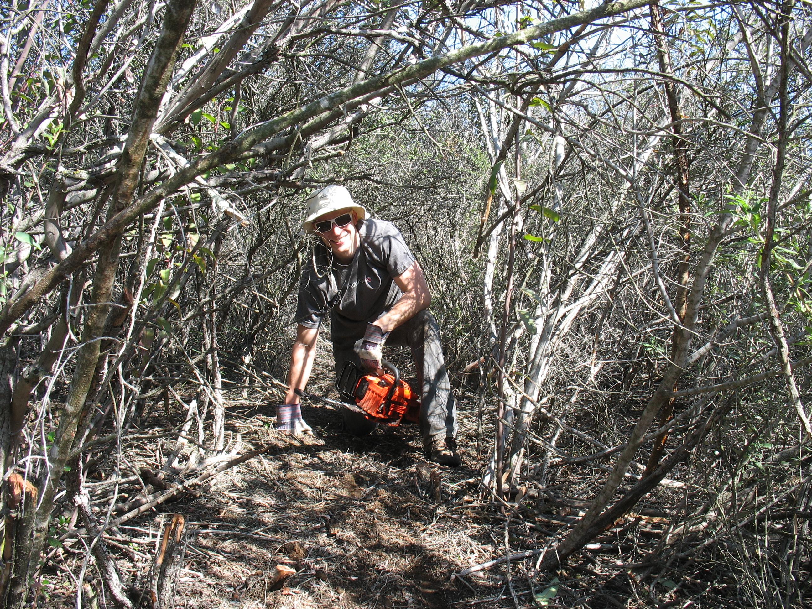
The second step was creating the ~120 m long trails to connect the sensors to their digitizers. We took special care to not damage root balls, to minimize the width of these trails, and to preserve the natural beauty of the landscape as much as possible (Figure 6). These trails were designed not to be perfectly straight (which could turn into a wind tunnel), but rather have small twists and turns throughout.

Figure 6. View looking northward along one of the created trails that connect the digitizer with the sensors. Great care was taken to create trails that blended into the natural beauty and diversity of the landscape. Photo taken February 12, 2010.

At the sensor locations, we created as many as four smaller trails (about 2' wide maximum) that were 50' long, radiating out from the sensor every 90 deg in azimuth.

Figure 7. Photo of UCSD undergraduate Rich Shelby standing beneath the path he created for one of the four 50' porous hoses. Photo taken February 12, 2010.

Along these trails we installed microporous irrigation "soaker hose" that we connected to the microbarometer. This porous hose reduces "wind noise," which is an important problem when a dense forest is not available to install the sensor in. In some cases, the chaparral canopy was high enough such that we could create covered trails through the brush (Figure 7).

Figure 8. SM05 sensor box. Photo taken June 3, 2010. The sensors are encased in boxes to protect them from rodents and the elements (Figure 8). The porous hoses are attached to the sides of the boxes. Signals and power cables run inside 3/8" liquid tight, steel-reinforced conduit between the sensor and digitizer boxes. Ten-foot ground rods are connected to the conduit/box couplers at both ends.

Figure 9. Photo of Michael Davis and Joel White next to the REF B digitizer box, solar panel, GPS, wireless radio antennas, and ground rod. Photo taken June 3, 2010.

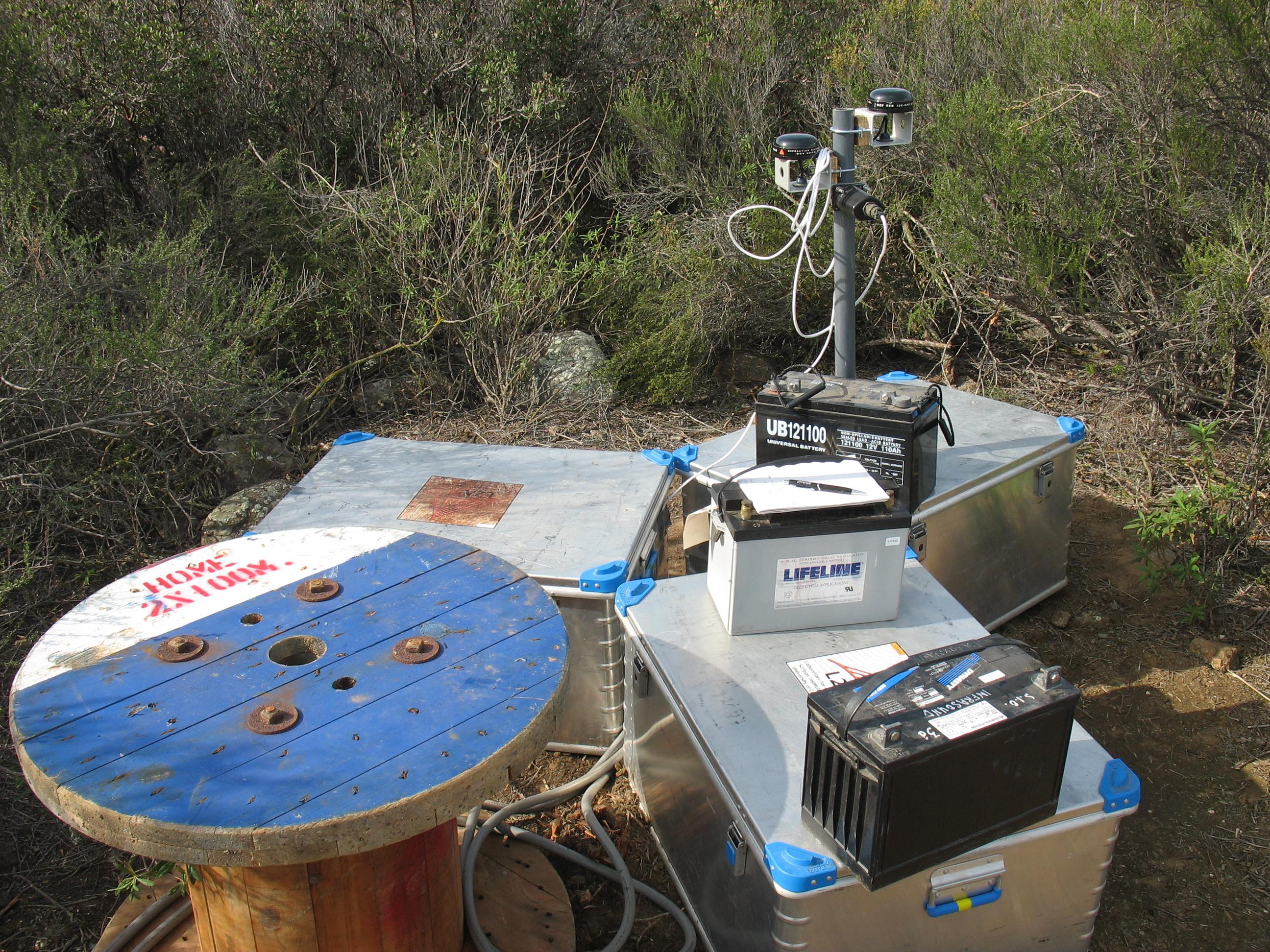
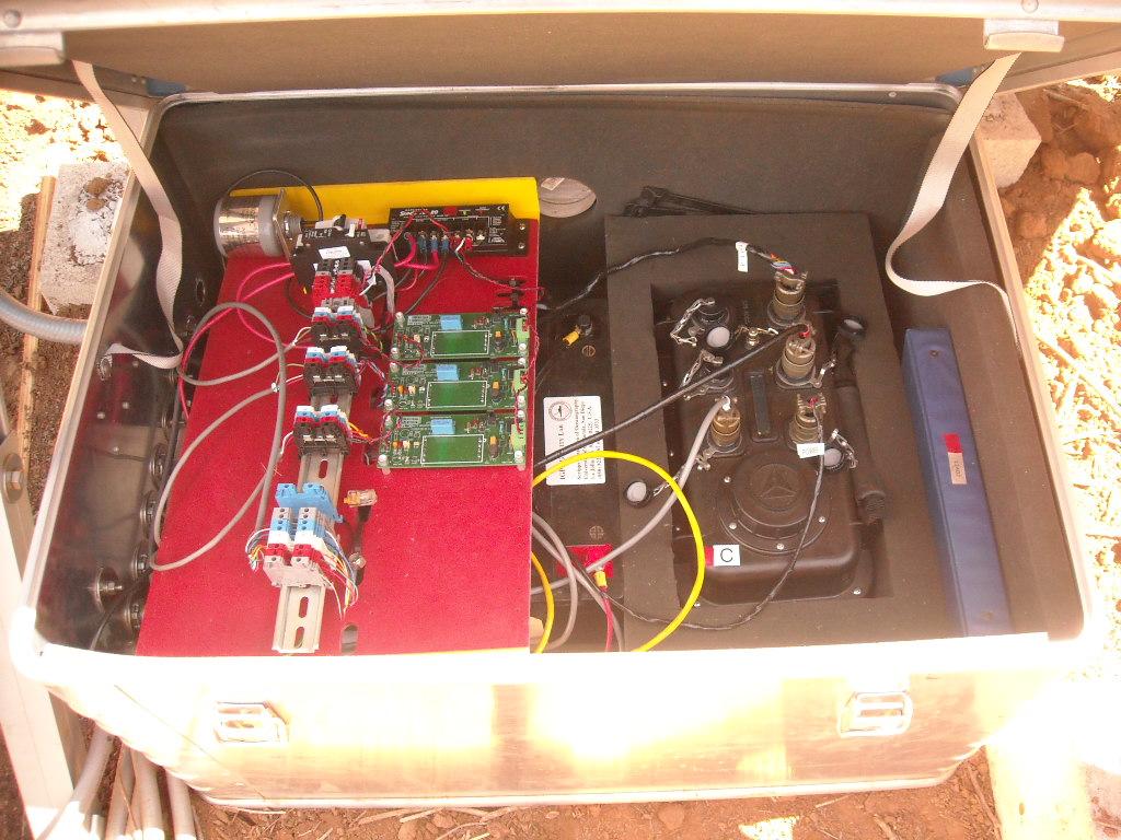
There are a total of three clusters of three sensors each. Each sensor is connected to a digitizer box, which also includes batteries, DC-DC converters, solar charge controller, and wireless radio (Figure 10). One box also configured with an outside temperature sensor and anemometer. The digitizer is a Reftek 130 running RTPD software to stream data to UCSD in real time over HPWREN. At our labs, we use home-grown software written by David Chavez to receive the streaming Reftek data. We then convert it to CSS 3.0 format for further analysis.

Figure 10. Inside of digitizer box. Photo taken June 3, 2010.

Figure 11. Photo of Joel White taking measurements at a wireless radio antenna with a differential GPS instrument. Photo taken June 3, 2010.

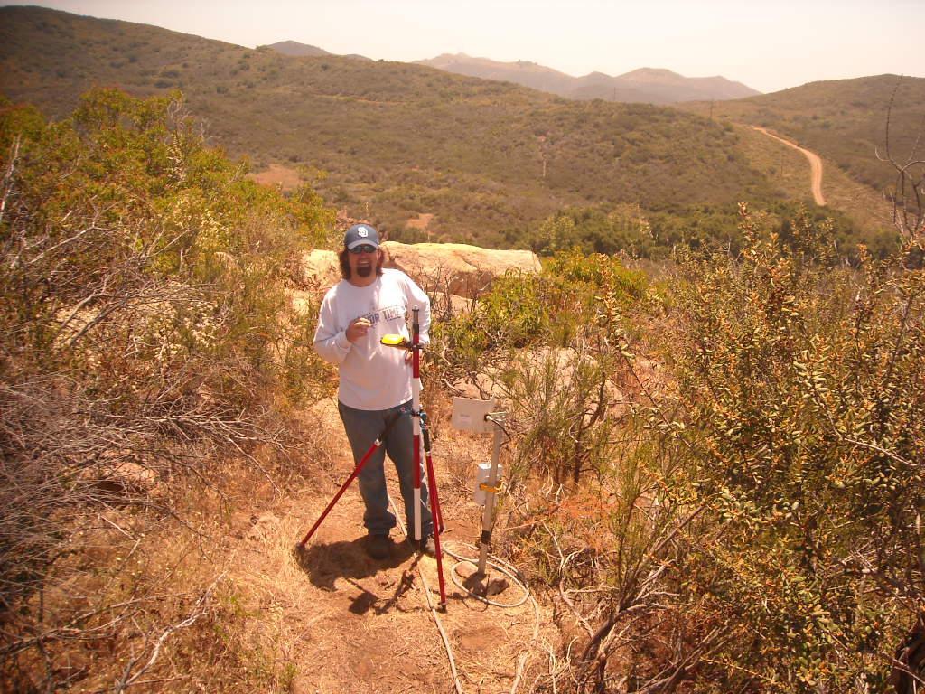
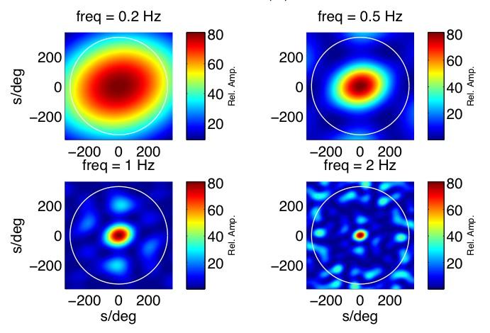
For each sensor, we used a differential GPS instrument to measure latitude, longitude, and elevation to obtain positioning information with an accuracy of about a few meters (Figure 11). This accuracy is useful for determining the direction from which infrasound signals cross the array (which points toward the source of the infrasound). The SMIAR array became fully operational on June 10, 2010.

Performance of the Array

The positioning of the sensors determines the potential of array processing software in determining the directions from which infrasound signals originate. A characteristic plot to evaluate this is the array response. Figure 12 shows the array response for SMIAR. This is really a polar plot where angle is the horizontal azimuth (north is up, east is to right) and radius is a measure of speed at which signals cross the array. The radius of the white circle is the typical infrasound apparent speed of 330 m/s. For smaller radii the apparent speed is greater. Greater speeds are expected for infrasound signals impinging down onto the array at some oblique angle (higher elevation angle). Perfect resolution is indicated by blue under the white circle and a single red dot in the center of the graph. If there are other red dots, then there will be "signal aliasing" for those signal directions and apparent speeds. Aliasing just means that there is not enough information to distinguish between the different "red-dot directions" for a continuous monochromatic signal. The array response for SMIAR is quite good for frequencies from 0.2 to 2 Hz.

Figure 12. Infrasound array response for frequencies of interest.

The wind speed at SMIAR is typically between 2-3 m/s during the day, with very little wind at night. This suggests that we will have a little more difficulty seeing infrasound signals during the day, but with the porous hoses, nine sensors, and array processing software, we should still be able to detect many daytime signals. Nighttime signals should be very easy to detect.

Figure 13. Six infrasound signals observed on SMIAR on June 10, 2010 (first day the array was fully operational). Peak-to-peak amplitude is 0.1 Pa. These signals are coming from 264 deg (west; see Figure 14).

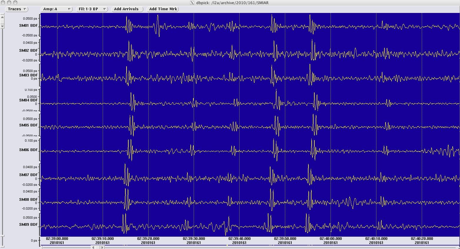
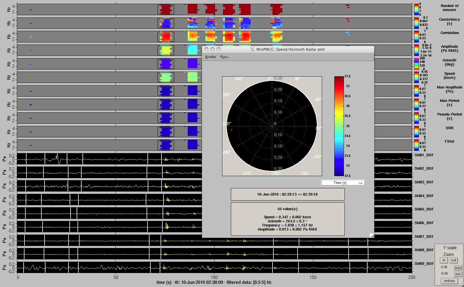
Immediately after the array became fully operational, we began seeing many interesting events from different directions. Figure 13 shows six such signals coming in around 7:30 PM local time. These signals are likely related to military training activities to the west of SMIAR. Such common activity is very useful in our research. We applied a traditional array processing method called Progressive Multi-Channel Correlation (PMCC; Figure 14). This method determined that the signal came across the array from an azimuth of 264 +/- 0.3 deg, which is almost due west. The apparent speed that the signal crossed the array was 347 m/s. The signals were very similar in appearance on all sensors (correlation of nearly 1). Finally, all the sensors contributed to the azimuth and speed determination, suggesting that the array is performing well.

Figure 14. Characteristic plot of array processing software PMCC. Time is on the x-axis. For the lower graphs, the time series is just repeated. For the upper graphs, the signal characteristics are plotted in different colors for time-frequency bins. The six different signals come from the same 264 deg azimuth (5th graph from top). Each of the signals comprises about 50 frequency-time bins (pixels). The azimuth variation in the pixels is 0.3 deg, which is quite good.

Figure 15 shows another 1-5 Hz signal coming from the southeast direction. Figure 16 shows microbarom waves crossing the array from the northwest. Figure 17 shows gravity waves crossing the array from the north. It is possible to distinguish the signal direction of these longer period gravity waves with the 700 m aperture SMIAR array because gravity waves travel much slower (~5-10 m/s) than infrasound waves (~300 m/s).

Figure 15. Time series plot showing a 1-5 Hz infrasound signal traveling across the array from the east.

Figure 16. Time series plot showing microbaroms in the 0.1-0.3 Hz infrasound band.

Figure 17. Time series showing ~700 s period gravity waves moving across SMIAR from the north.

Conclusions

SMIAR can detect and characterize faint infrasound signals with quite good directional resolution in the 0.2 to 10 Hz range. It can also detect and characterize long period gravity waves. The array is well positioned, with respect to the other SoCal infrasound arrays, to study regional infrasound sources and propagation characteristics. The relatively large number of microbarometers in the array also permits testing of advanced array processing techniques.

Acknowledgements

We thank the SMIAR field crew for their efforts: Rich Shelby, David Bellanger, Charles Way, Michael Davis, Joel White, Bienvenido Landrito, Clint Coon, John Lyons, and Pablo Bryant. We thank Michael Davis and Joel White for their efforts as our SMIAR electrical and mechanical engineers. We thank John Lyons, Mike Kirk, Clint Coon, Glenn Sasagawa, Glen Offield, and Pablo Bryant for providing lab assistance and engineering advice. We thank Ian Billings for assistance with installing the Reftek. We thank Redick Edwards for assistance in hiring temporary employees. We thank David Chavez for creating the software and managing the real-time data streams. We thank Hans-Werner Braun and the NSF-funded High-Performance Wireless Research and Education Network (HPWREN) for providing us with wireless data access. We are indebted to Matt Rahn, John Kim, and the San Diego State University Field Stations Program for permitting usage of Santa Margarita Ecological Reserve.

Additional Information

For more information, contact Kris Walker (walker @ ucsd.edu) or Michael Hedlin (mhedlin @ ucsd.edu). This document was created on June 18, 2010.

Main HPWREN web site (includes information for acknowledgments/disclaimers and feedback/contact)